
On my way home, I noticed a few mushrooms that had sprung up after the rain. They were perfect and intact because everyone knew they were poisonous.
— Paulo Coelho
With all of the rain lately, I’ve noticed quite a few mushrooms on my daily walks. Some are tall , balancing caps on top of slender stalks, resembling an art instillation along the trail.

Others hug close to the ground, their gills pressed to the soil as though they are afraid of heights.

Some wear brightly-colored caps that stand out on the woodland floor.

Many are beautiful.
All are interesting.
And some are deadly.
Do YOU know which ones are poisonous?
Starting With the Data
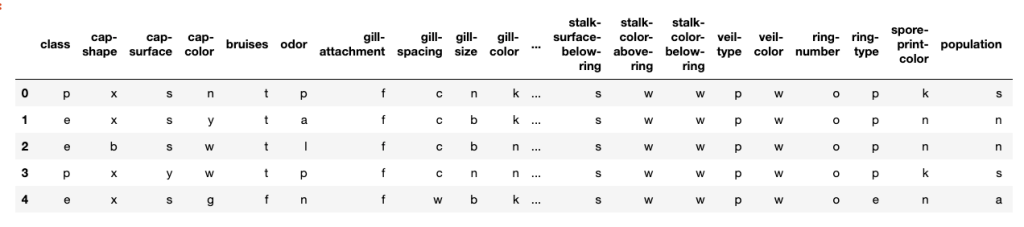
I started by downloading the mushroom.csv from Kaggle. This dataset contains 8,124 hypothetical observations of 23 different mushroom species found in North America. Each observation is described by 22 different features (including shape, color, rings, odor, etc.) and is classified as either edible (yum!) or poisonous (uh oh!).
My goal is to use this labeled dataset to create a model that can be used to determine if you can make a mushroom omelet or if you should keep your distance.
I am going to be using be using a logistic regression model. Before I go any further, I need to check to see if the target variable (class) is balanced. If it is not, I will need to apply a resampling technique in order to have accurate results.
df['class'].value_counts(normalize=True)
We’re in luck! 52% are classified as edible and 48% are deemed poisonous. This means the classes are already balanced.
Next, I have some decisions to make. I decide that I only want to focus on features that are ones that a non-expert could distinguish in the field. Based on this, I’m going to limit my features to only cap-shape, cap-color, gill-color, odor (although I do have some doubt on this one when I consult the documentation and see descriptors of “fishy” and “foul”) and habitat.
I also start to think about what preprocessing I will need to do. All of the data is currently categorical and encoded as strings. In order to perform logistic regression, I will need to make these numerical.
I will use SciKit-learn’s LabelEncoder on the target in order to transform it into 0s and 1s before splitting the data because it will not lead to any data leakage. With the features, I will need to include OneHotEncoder into my pipeline for cross validation in order to prevent data leakage.
#split the features and target
y = df['class']
X = df.drop('class', axis=1)

#select only the desired columns
X = X[['cap-shape', 'cap-color','gill-color','odor','habitat']]

#transform the target
le = LabelEncoder()
y = le.fit_transform(y)
Once encoded, 1 indicates poisonous and 0 corresponds to edible.
Then, before anything else is done, it’s time to train_test_split and set aside the validation data. It’s always a good idea to check the shape of the data to make sure that it’s what you expect.
X_train, X_test, y_train, y_test = train_test_split(X,
                                                    y,
                                                    random_state=44,
                                                    stratify=y)
X.shape, y.shape

((8124, 5), (8124,))


X_train.shape, X_test.shape, y_train.shape, y_test.shape

((6093, 5), (2031, 5), (6093,), (2031,))
Training the Model
Because all of the predictors will be one hot encoded, there is no need to scale this data. As a result, the pipeline is quite simple.
pipeline = Pipeline(steps = [['ohe', OneHotEncoder(handle_unknown='ignore')],
                             ['classifier', LogisticRegression(random_state=44,
                             max_iter=1000)]])
Next, I will use GridSearch and cross validation in order to access the performance of the model and select the best value for C. This is a regularization hyperparameter, where the smaller the value, the stronger the regularization.
stratified_kfold = StratifiedKFold(n_splits=5,
                                       shuffle=True,
                                       random_state=44)


param_grid = {'classifier__C':[0.001, 0.01, 0.1, 1, 10, 100, 1000]}

grid_search = GridSearchCV(estimator=pipeline,
                           param_grid=param_grid,
                           scoring=['neg_log_loss', 'f1'],
                           cv=stratified_kfold,
                           n_jobs=-1,
                           refit='neg_log_loss',
                           return_train_score=True)

grid_search.fit(X_train, y_train)
This told me that the ideal value for C is 1000, indicating that not much regularization needs to be done. I quickly examine the metrics for the cross-validated model with C=1000:
param_classifier__C                             1000
params                       {'classifier__C': 1000}
split0_test_neg_log_loss                 -0.00642688
split1_test_neg_log_loss                  -0.0074723
split2_test_neg_log_loss                  -0.0204453
split3_test_neg_log_loss                  -0.0160083
split4_test_neg_log_loss                  -0.0124653
mean_test_neg_log_loss                    -0.0125636
std_test_neg_log_loss                     0.00524552
rank_test_neg_log_loss                             1
split0_train_neg_log_loss                  -0.011294
split1_train_neg_log_loss                 -0.0112726
split2_train_neg_log_loss                -0.00849542
split3_train_neg_log_loss                -0.00930276
split4_train_neg_log_loss                -0.00986136
mean_train_neg_log_loss                   -0.0100452
std_train_neg_log_loss                    0.00110025
split0_test_f1                              0.998296
split1_test_f1                              0.997451
split2_test_f1                              0.993139
split3_test_f1                              0.995723
split4_test_f1                              0.997438
mean_test_f1                                0.996409
std_test_f1                               0.00183693
rank_test_f1                                       1
split0_train_f1                             0.996583
split1_train_f1                             0.996157
split2_train_f1                             0.997226
split3_train_f1                              0.99744
split4_train_f1                             0.997012
mean_train_f1                               0.996884
std_train_f1                              0.00046093
Looking at the log-loss, I notice that the values are consistent across the splits and that the loss is slightly larger for the test set, which is not surprising (remember to consider the opposite of these values as they’re listed). All of the log-loss seems quite small, indicating a small error rate between the predicted class and the actual class.
Next, I look at the f1 scores, which are the harmonic mean of precision and recall, giving a quick idea of overall performance. Again, these are consistent between folds (which is also verified by the very small standard deviations). Additionally, the f1 scores are quite high for both the train and test sets. I decide to proceed with this model.
#Fitting a final model on the entire train set

pipeline_final = Pipeline(steps = [['ohe', OneHotEncoder(handle_unknown='ignore')],
                             ['classifier', LogisticRegression(random_state=44,
                             max_iter=1000, C=1000)]])

best_model = pipeline_final.fit(X_train, y_train)

y_pred = best_model.predict(X_test)
pd.Series(y_pred).value_counts()

#predictions
0    0.519449 #edible
1    0.480551 #poisonous

#actual
e    0.517971 #edible
p    0.482029 #poisonous
Wow! On first glance, that seems like an awesome result! But with data, as with mushrooms, you don’t want to rush to judgment too quickly as the results could be disastrous. So, let’s look a little deeper.
Evaluating the Model
My first step is to make a quick histogram of the probabilities (not just the actual classes) that the model assigned to each data point.
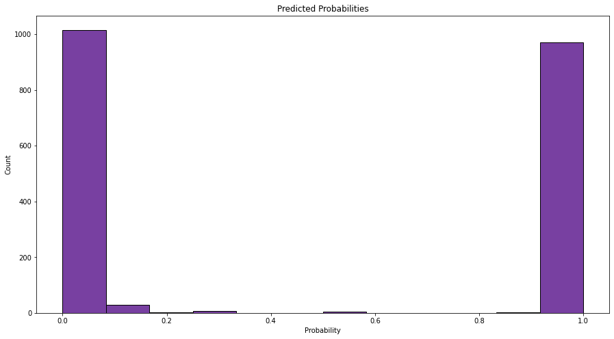
These values are clustered around 0 and 1, which means that the model is quite certain about its predictions. We can also see the roughly 50-50 split that we saw with the actual classifications. Looking good so far.
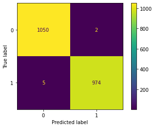
Next, I dig deeper into the metrics by plotting a confusion matrix.
plot_confusion_matrix(pipeline_final, X_test, y_test);
Let’s use this to get three important metrics.
Accuracy
Accuracy is the total number of correct predictions out of the total number of predictions.
2024/(2024+7) = 99.66%
This means the model was correct was correct 99.66% of the time.
Precision
Precision is how many are actually positive (which in this case, is poisonous or 1) out of the ones that the model predicted were positive.
974/(974+2)= 99.80%
This means that of the mushrooms the model indicated were poisonous, 99.8% actually are.
Recall
Recall is out of the actual positive cases (again, poisonous or 1), how many the model recognized as positive.
974/(974+5) = 99.48%
This means that the model picked up on 99.48% of the poisonous mushrooms. Which doesn’t seem so bad unless you happen to be one of those 0.52% of people that inadvertently makes a deadly omelet.
Precision/Recall Tradeoff
This is one of those situations where it is much more preferable to have false positives (a perfectly harmless mushroom is labeled as poisonous) than false negatives (you think a deadly mushroom is harmless). It’s okay if you skip eating a mushroom that won’t hurt you. but it’s a pretty bad day if you eat one that will cause your limbs to fall off of your body.
Adjust the Threshold
As the model is written, it will interpret any probability below 0.5 as a harmless blob of fungi. But because a false negative here is so dangerous, I’m going to set that threshold to 0.1 so that any data points with above a 10% probability of being poisonous will be put into the “Don’t eat!” bin.
def final_model_func(model, X):
    probs = model.predict_proba(X)[:,1]
    return [int(prob > 0.01) for prob in probs]

threshold_adjusted_probs = pd.Series(final_model_func(pipeline_final, X_test))
threshold_adjusted_probs.value_counts(normalize=True)

#new predictions
1    0.520433 #edible
0    0.479567 #poisonous

#original predictions
0    0.519449 #edible
1    0.480551 #poisonous
We can see that by doing that, the percentage of mushrooms classified as poisonous increased slightly. Now, let’s see what happened to our metrics.
print(f"Accuracy: {accuracy_score(y_test, threshold_adjusted_probs)}")
print(f"Precision: {precision_score(y_test, threshold_adjusted_probs)}")
print(f"Recall: {recall_score(y_test, threshold_adjusted_probs)}")

Accuracy: 0.9615952732644018
Precision: 0.9262062440870388
Recall: 1.0
By changing the threshold, the accuracy and the precision both dropped. This is because the model is now classifying some harmless fungi as bad guys. But the tradeoff is worth it because that recall value of 1 says that we’re not going to accidentally ingest a poisonous mushroom (as long as we listen to the model, that is!)
Interpreting the Model
Let’s look at the features with the largest or smallest coefficients, as these are the characteristics that are the most impactful on the decision.
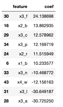
That’s a little tricky to interpret since the features have been one hot encoded. Let’s remind ourselves what the general categories are.
x0 = ‘cap-shape’
x1 = ‘cap-color’
x2 = ‘gill-color’
x3 = ‘odor’
x4 = ‘habitat’
Looking at the most impactful coefficients, x0 does not appear, so cap shape is not a great predictor of the presence of poison. The rest can be attributed to cap-color (10%), gill-color (20%), odor (60%) and habitat (10%). So, it looks like your nose knows if a mushroom will harm you.
This can be confirmed with the following graph, which clearly shows that odor alone is a pretty good separator of poisonous vs. tasty shrooms.
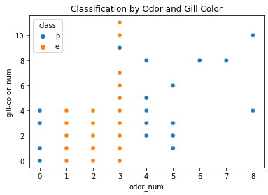
But that’s still not super helpful. After all, what DO the dangerous ones smell like?
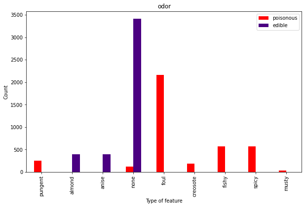
Well, that’s actually pretty handy After all, if a mushroom smells pungent, foul, fishy, tar-like (creosote) or musty, it’s not exactly begging to be put on your pizza. Buy you might need to look out for those spicy ones and the ones with no discernible odor.
And in case you want to become your own mushroom classification machine, here are the other characteristics.
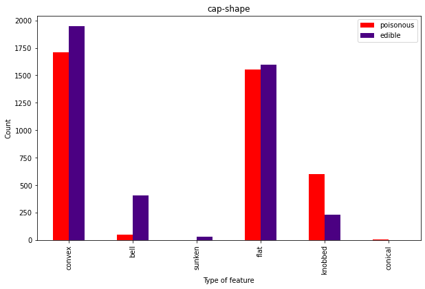
As expected from the coefficients, cap shape isn’t super useful since it doesn’t seem to separate the classes well.
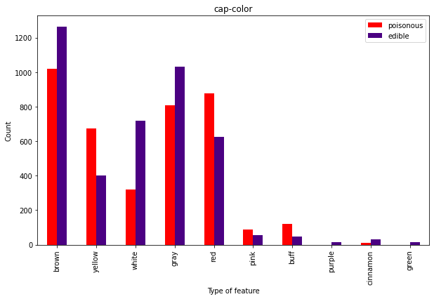
Overall, the caps don’t seem super useful here.
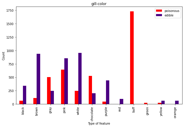
Now we’re talking. You may like the buff guys, but don’t eat the buff fungis:)
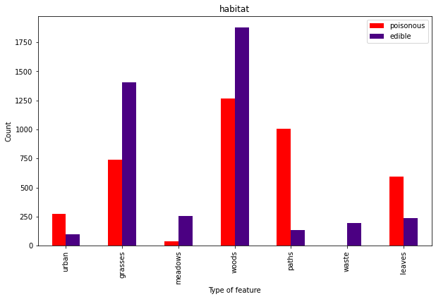
Mental note – don’t eat mushrooms from a pile of leaves on an urban path.

Lesson of the Day
I’m finally getting the picture of how cross validation, pipeline and model selection all work together. Whew.

Frustration of the Day
I finish a project. I feel good about it for a couple hours. I learn new things. I feel ashamed of some of the choices I made on my project.

Win of the Day
The frustration above is a sign I’m learning:)

Current Standing on the Imposter Syndrome Scale
3/5
Doing okay at the moment.
