
“If you never try, you’ll never know.”
The Situation
The developer of a phone-based game is concerned about the retention rate of customers who download the game after they saw this graphic in a company presentation.
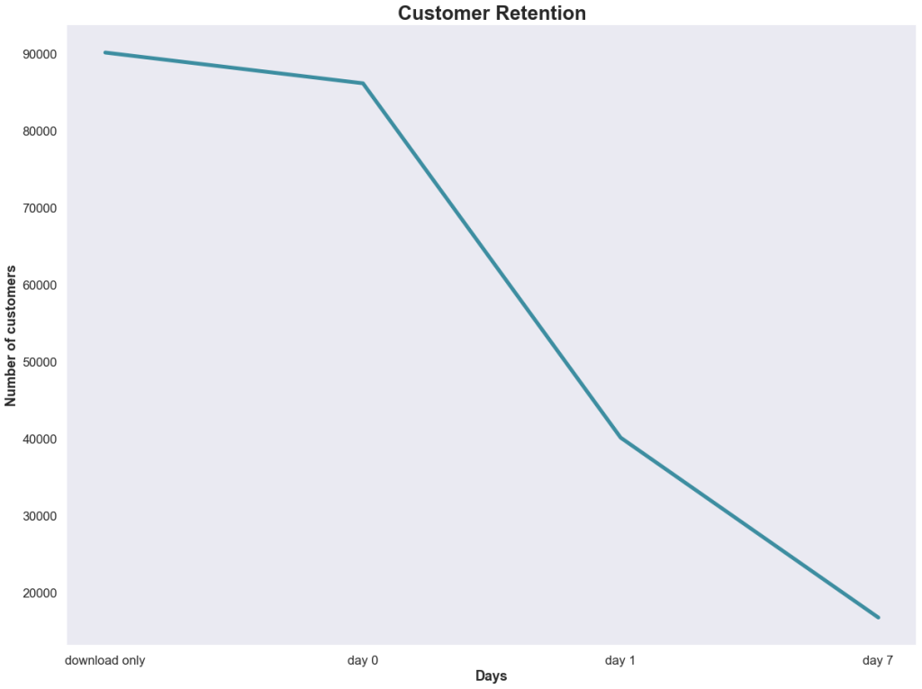
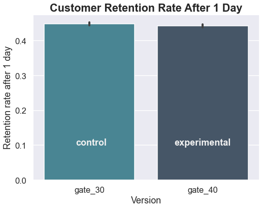
The developer was especially concerned about the customers that churned after the first day. This indicated that they were interested enough in the game’s concept to try it out, but that something in the game failed to meet their expectations.
Hypothesizing that the beginning of the game was too easy, thus failing to keep the players’ attention, the developer proposed an A/B test where customers would be randomly selected to either begin the game at gate 30 (the previous starting point) or the more difficult gate 40 (the new starting point).
A test is set up and the data are collected.
Examining the Data
Data were collected from 90,189 customers that downloaded the game.
df = pd.read_csv('cookie_cats.csv')
df.head()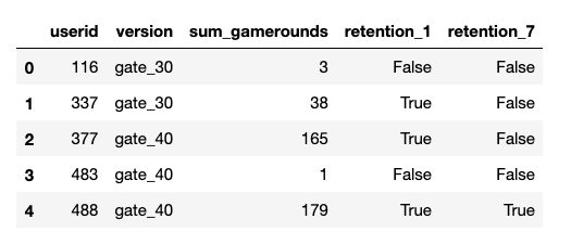
Along with the A/B version and the retention at day 1 and 7, the total number of games played by the customer within the 7-day period was also collected.
(df['sum_gamerounds'] == 0).sum()
3994
There were 3,994 players that downloaded the game and did not play.
Before any further analysis is done, it makes sense to check for any unusual values.
df[df['sum_gamerounds']>2000]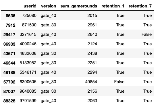
Wow! According to this, user #6390605 managed to play 49,854 games in a week! While that may technically be possible, it certainly appears to be an error, especially since the next highest value is 2,961. I will go ahead and remove this value before doing any other analysis.
#Looking at the distribution of players who completed 200 or fewer games
fig,ax = plt.subplots(figsize=(15,8))
df.groupby('sum_gamerounds')['userid'].count().plot(color=NEUTRAL)
plt.xlabel('Number of games played')
plt.ylabel('Count of players')
plt.title('Number of Games Played', fontweight='bold', size='large')
plt.xlim(0,200);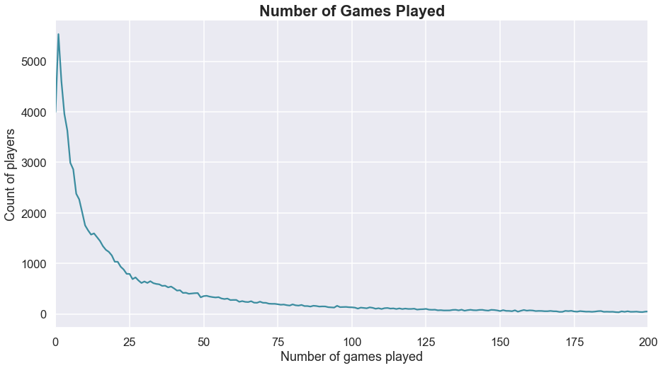
Before running the statistical tests, it also makes sense to check the retention values.
x = ['download only', 'day 0', 'day 1', 'day 7']
y1 = (
    [control.shape[0],
     (control['sum_gamerounds'] != 0).sum(),
     control['retention_1'].sum(),
     control['retention_7'].sum()]
)
y2 = (
    [exp.shape[0],
     (exp['sum_gamerounds'] != 0).sum(),
     exp['retention_1'].sum(),
     exp['retention_7'].sum()]
)

fig,ax = plt.subplots(figsize=(20,15))
plt.plot(x,y1, color=NEUTRAL, linewidth=5, label='control')
plt.plot(x,y2, color=DARK_GRAY, linewidth=5, label='experimental')
plt.xlabel('Days', fontweight='bold')
plt.ylabel('Number of customers', fontweight='bold')
plt.title(
    'Customer Retention A/B Test',
    fontsize='x-large',
    fontweight='bold'
)
plt.grid(False)
plt.legend();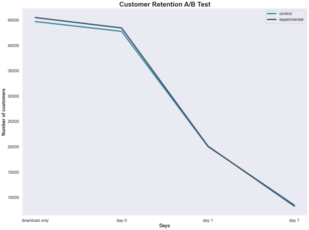
Well, that’s not looking promising for the developer’s hypothesis that changing the initial gate from 30 to 40 would increase retention. But let’s make sure using some statistical testing.
Setting the Hypotheses
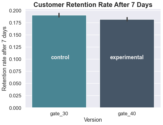
The developer’s hypothesis is that the new version (gate 40) will perform better than the previous version (gate 30) on retaining customers at the 7-day mark. This leads to a one-tailed test where:
H0: gate_40 <= gate_30
or gate_40 – gate_30 <= 0
HA: gate_40 > gate_30
or gate_40 – gate_30 > 0
The confidence level will be set at 0.05.
Only the proportions of customers retained at the 7-day point will be considered.
Testing the Hypothesis
#Get a series for the retention values at day 7 for the control and
#experimental groups
control_results = df[df['version'] == 'gate_30']['retention_7']
exp_results = df[df['version'] == 'gate_40']['retention_7']

#Get the number of observations in each group
n_con = control_results.count()
n_exp = exp_results.count()

#The successes are the number of true values
successes = [control_results.sum(), exp_results.sum()]
nobs = [n_con, n_treat]

#Perform a one-tailed z-test using the proportions
z_stat, pval = proportions_ztest(successes, nobs=nobs, alternative='larger')
(lower_con, lower_exp), (upper_con, upper_exp) = proportion_confint(
    successes,
    nobs=nobs,
    alpha=0.05
)

print(f'z statistic: {z_stat:.2f}')
print(f'p-value: {1-pval:.3f}')
print(f'ci 95% for control group: [{lower_con:.3f}, {upper_con:.3f}]')
print(f'ci 95% for experimental group: [{lower_exp:.3f}, {upper_exp:.3f}]')

z statistic: 3.16
p-value: 0.999
ci 95% for control group: [0.187, 0.194]
ci 95% for treatment group: [0.178, 0.186]
The p-value is (much!) greater than the critical value of 0.05, which means we fail to reject the null hypothesis that the retention rate for gate 40 is less than or equal to that of gate 30. The confidence intervals do not overlap and show that gate 30 has a higher retention rate.
To be even more confident in this conclusion, bootstrapping can be performed. Bootstrapping using random sampling with replacement to simulate repeated experiments. In this case, 10,000 simulated experiments will be performed with the data.
#Using bootstrapping to sample the data

differences = []
control_results = []
exp_results = []
size = df.shape[0]

for i in range(10_000):
    sample = df.sample(size, replace=True)
    results = sample.groupby('version')['retention_7'].value_counts()
    control_ctr = results['gate_30'][True]/results['gate_30'].sum()
    exp_ctr = results['gate_40'][True]/results['gate_40'].sum()
    control_results.append(control_ctr)
    exp_results.append(results['gate_40'][True].sum())
    differences.append(exp_ctr - control_ctr)

fig,ax = plt.subplots(figsize=(15,8))
sns.kdeplot(control_results, label = 'control', color=DARK_GRAY)
sns.kdeplot(exp_results, c=NEUTRAL, label='experimental')
plt.title(
    'Distributions of Control and Experimental Samples',
    fontweight='bold',
    fontsize='large'
)
plt.legend();
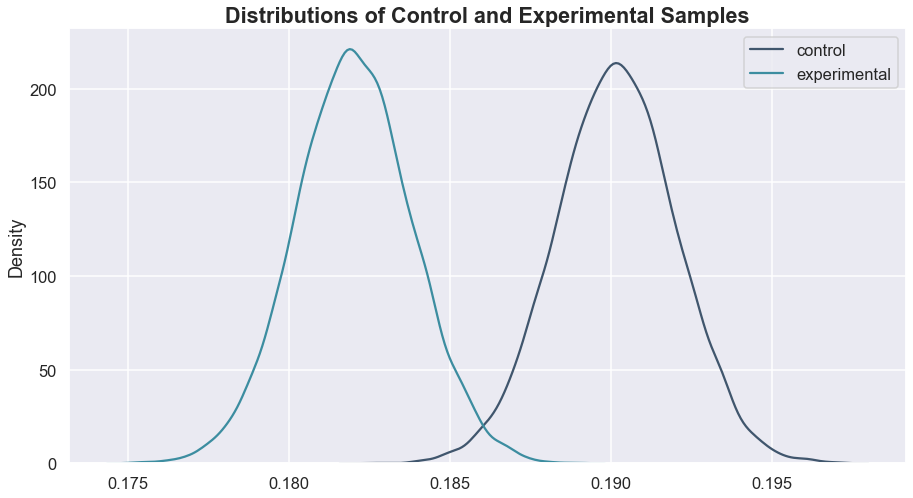
Looking at that, it is apparent that changing the gate to 40 is not a good idea, as almost the entire experimental distribution is below the control, indicating a lower retention at the 7-day point.
Another way that we can look at this is to compare the differences (gate 40 – gate 30) from the bootstrapped samples against a null distribution centered at 0 (this would be the most extreme case in the null hypothesis stated above).
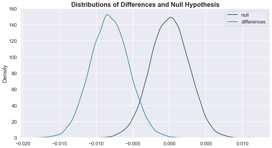
Remember, we’re testing to see if the differences are larger than 0. This doesn’t look very promising at all.
Again, using statsmodels:
pval = ztest(differences, null_hypothesis, alternative='larger')

pval
1.0
Based on the p-value and the graphs, we can be confident in our conclusion that gate 40 will not result in a higher retention rate at day-7 than gate 30.
Trying a Different Approach
When faced with the disappointing conclusion, the game developer had one more idea – “Maybe the retention isn’t better, but perhaps the gate change impacted how many games customers completed.”
This time, we’ll use a two-tailed test, not assuming the direction of any difference, with a null hypothesis that the two versions have the same number of games played.
#bootstrapping again for the number of rounds
control_results_rounds = []
exp_results_rounds = []
size_rounds = df.shape[0]

for i in range(10_000):
    sample_rounds = df.sample(size_rounds, replace=True)
    results_rounds = sample_rounds.groupby('version')['sum_gamerounds'].mean()
    control_rounds = results['gate_30']
    exp_rounds = results['gate_40']
    control_results_rounds.append(control_rounds)
    exp_results_rounds.append(exp_rounds)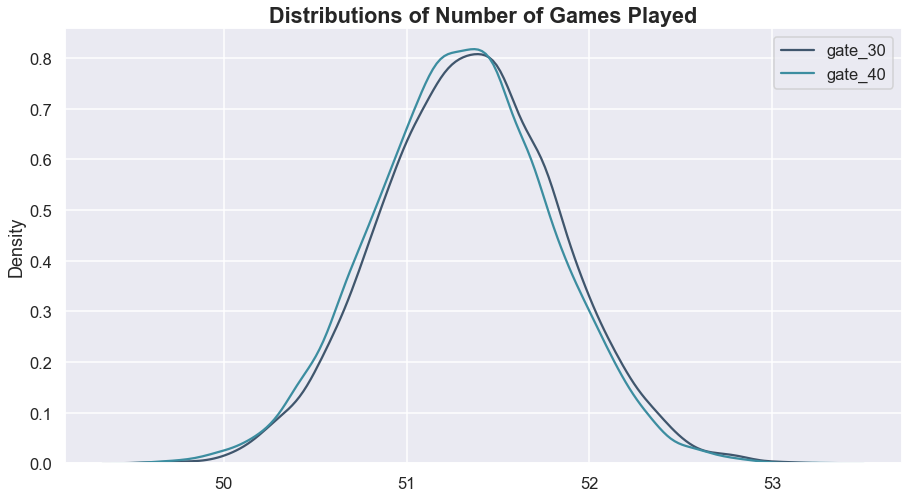
Both the visualization and the p-value confirm that we cannot determine that the gate change led to a difference in the number of games played.
Conclusion & Recommendations
The company should not make the change to starting at gate 40, as this led to a decrease in retention at the 7-day point. In fact, they may want to experiment with a change that makes the beginning of the game slightly easier rather than harder since gate 30 led to a better retention rate.
Based on the number of games played, it seems that the starting gate influences how likely someone is to stick with the game over the long-term, but does not impact the frequency that they play.

Lesson of the Day
I learned about the validation argument in pandas when merging dataframes. Pretty cool and a reminder to look for solutions like this before making things harder on myself.

Frustration of the Day
Job hunting is rough, y’all.

Win of the Day
Major compliment from the bootcamp I just graduated from. I’m going to keep that one close to me right now.

Current Standing on the Imposter Syndrome Scale
1-5/5
Depends on the hour.
